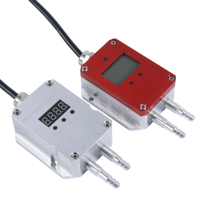
What Does 0.075% Accuracy Mean for a Differential Pressure Transmitter?

Maximum reference error = Full-scale span × 0.00075

When a differential pressure transmitter is specified with 0.075% FS accuracy, its maximum reference error is typically plus or minus 0.075% of the stated full-scale span under defined reference conditions. For a 0–100 kPa range, the calculation is 100 kPa × 0.00075 = 0.075 kPa, so the reference error is ±75 Pa. It is not automatically 0.075% of the pressure being measured at that moment. This distinction matters because the same ±75 Pa represents 0.075% of a 100 kPa span but 0.75% of a 10 kPa reading. Before comparing transmitters, confirm what the manufacturer means by full scale, whether the specification applies to the sensor URL or the configured span, and which error components are included.

Key Takeaways

• A 0.075% FS specification normally means a maximum reference error of ±0.00075 multiplied by the defined span.

• For a 0–100 kPa transmitter, 0.075% FS equals ±75 Pa.

• Percent of full scale is not the same as percent of the current reading.

• “Accuracy” may include linearity, hysteresis, and repeatability, while temperature effects, static-pressure effects, long-term drift, and output errors may be specified separately.

• Turndown can make a fixed error much larger as a percentage of the configured working span.

• The lowest headline accuracy is useful only when the pressure range, installation, calibration, and application also support it.

What Does 0.075% Accuracy Mean?

The notation “0.075% FS” expresses error as a percentage of full scale or full-scale span. Converting the percentage to a decimal gives 0.00075. Multiply that number by the span defined in the datasheet to obtain the maximum reference error in engineering units.

For example, if the specified span is 40 kPa:

40 kPa × 0.00075 = 0.03 kPa = 30 Pa

Because measurement error can be positive or negative, the result is written as ±30 Pa. At an ideal differential pressure of 20 kPa, an instrument operating within this reference-accuracy limit could indicate from 19.970 to 20.030 kPa under the stated reference conditions.

The percentage does not usually follow the current reading. A 40 kPa full-scale instrument still has a ±30 Pa reference-error band at a 5 kPa measurement if its specification is strictly 0.075% FS. Relative to that 5 kPa reading, ±30 Pa is ±0.6%. This is why percent-of-span accuracy becomes increasingly important at the lower end of a range.

It is also important to distinguish standard accuracy from an optional high-accuracy configuration. One model may be supplied as ±0.1% FS by default and offer ±0.075% FS as an option. Another model may achieve ±0.075% FS only for specified ranges, while its lowest range carries a different value. The ordering code and range-specific datasheet table—not the product-family headline—determine what will be delivered.

0.075% Accuracy Calculation Examples

The following examples assume the manufacturer defines accuracy as ±0.075% of the listed full-scale span. They do not include temperature, static-pressure, installation, drift, or calibration-system effects.

The same method works for any engineering unit. For a 0–250 mbar range, the maximum reference error would be 250 mbar × 0.00075 = ±0.1875 mbar. Keep the input and result in consistent units.

For a bidirectional range, calculate the span rather than using only the positive endpoint. A −100 to +100 kPa range has a 200 kPa span. At 0.075% of span, its maximum reference error is therefore:

200 kPa × 0.00075 = ±0.15 kPa = ±150 Pa

This bipolar example is a common source of underestimation. Using 100 kPa as “full scale” would ignore half of the calibrated interval.

Is 0.075% Based on Full Scale, Span or Reading?

There is no safe answer without reading the exact accuracy statement. Instrumentation datasheets use several related terms, and the calculation can change substantially depending on which term appears in the formula.

Full scale (FS) often means the complete measurement range stated for the instrument. For a 0–100 kPa range, the full-scale span is normally 100 kPa. For a −25 to +25 kPa range, it is 50 kPa. However, some manufacturers use “full scale,” “full-scale output,” and “span” differently, so the definition section of the datasheet takes priority.

Span is the difference between the upper range value and lower range value:

Span = URV − LRV

A transmitter calibrated from 20 to 100 kPa therefore has an 80 kPa span, even though its upper value is 100 kPa.

URL, or upper range limit, is the highest measurement limit supported by a particular sensor capsule or range code. It describes sensor capability, not necessarily the configured operating range. A transmitter with a 100 kPa URL might be calibrated for 0–10 kPa, producing a 10:1 turndown.

Calibrated span is the configured measurement interval between the lower range value and upper range value. For a 4–20 mA output configured as 0–10 kPa, the calibrated span is 10 kPa, even if the sensor URL is 100 kPa.

Percent of reading changes with the measured value. If a specification were ±0.075% of reading, the error at a 10 kPa reading would be ±7.5 Pa, while at 100 kPa it would be ±75 Pa. By contrast, ±0.075% of a 100 kPa full-scale span remains ±75 Pa throughout the range.

Some smart-transmitter specifications use a formula that combines a base percentage with a URL-to-span term. Others quote a percentage of calibrated span only within a specified turndown. Therefore, do not compare two “0.075%” claims until you have checked the reference basis, range limits, turndown conditions, and included error terms in both datasheets.

What Is Included in an Accuracy Specification?

“Accuracy” is often shorthand for reference accuracy, but there is no universal list of included effects. Many transmitter specifications combine terminal-based linearity, hysteresis, and repeatability under defined reference conditions. Zero and span settings may be treated separately, and environmental or installation effects are commonly listed in other sections.

Linearity

Linearity describes how closely the transmitter’s output follows the ideal straight-line relationship between differential pressure and output. A linearity error can be small near calibration points yet larger between them. Datasheets may calculate it using independent linearity, best-fit straight line, or terminal-based methods; these methods can produce different numerical results.

Hysteresis

Hysteresis is the difference in output when the same pressure point is approached from increasing and decreasing directions. For example, the indicated value at 50 kPa may differ slightly depending on whether pressure was raised from 25 kPa or lowered from 75 kPa. This is why a proper verification test includes both ascending and descending pressure cycles.

Repeatability

Repeatability is the instrument’s ability to return the same output when the same input is applied repeatedly under unchanged conditions. Good repeatability is essential for stable control and reliable trending, but it does not prove that the result is close to the true reference value. An instrument can repeat a biased value consistently.

Zero and Span Error

Zero error shifts the entire output curve up or down. Span error changes the slope between the lower and upper range points. Mounting position, manifold operation, pressure cycling, and commissioning conditions can introduce or reveal these errors. A zero trim can correct an offset, but it cannot compensate for every nonlinearity, temperature effect, or static-pressure effect.

Reference accuracy should therefore be treated as one part of an uncertainty budget, not as a promise that every installed reading will remain within ±0.075% under all operating conditions. Check whether the specification includes the sensing element only, terminal output, digital output, or the complete analog signal path. Analog-to-digital conversion, digital-to-analog conversion, and control-system input accuracy can add further uncertainty.

Reference Accuracy vs Total Installed Error

Reference accuracy is normally established under controlled conditions: a defined ambient temperature, stable power supply, specified mounting, limited static pressure, and a calibrated reference source. Total installed error reflects what happens in the real process. It can be larger because it includes effects beyond the laboratory reference-accuracy test.

Key contributors include:

• Ambient and process temperature: Electronics, sensing diaphragms, fill fluid, capillaries, and impulse lines can respond to temperature changes. A transmitter’s compensated temperature range and separate thermal-effect specification are therefore important.

• Static line pressure: High common pressure on both sides of a DP sensor can shift zero or span even when the differential pressure is small.

• Long-term drift: Sensor and electronic characteristics can change gradually between calibration intervals.

• Turndown: If error is tied to the sensor URL or a fixed range, reducing the configured span increases error as a percentage of the working span.

• Impulse-line installation: Unequal line lengths, trapped gas in liquid service, liquid heads in gas service, plugging, leaks, and temperature differences can create false differential pressure.

• Zero shift: Mounting orientation, remote seals, unequal wet legs, and static-pressure application can move the zero point.

• Calibration equipment uncertainty: The pressure controller, reference standard, electrical meter, connections, and test procedure must be more capable than the transmitter being evaluated.

A practical error budget should also consider the output and receiving device. For a 4–20 mA loop, include the transmitter’s analog output performance and the PLC or DCS input-card uncertainty when these are not already included. For a digital HART reading, confirm whether the stated reference accuracy applies to the digital process variable, the analog output, or both.

The point is not that a 0.075% instrument will perform poorly in the field. It is that selecting a precise sensor is only one step. Correct range selection, installation, equalization, temperature management, commissioning, and periodic verification are what allow the application to benefit from that precision.

How Static Pressure Affects Differential Measurement

Differential pressure is the difference between the pressure applied to the high-pressure port and the pressure applied to the low-pressure port:

DP = P-high − P-low

In a high-static-pressure application, both ports may be exposed to a very large common pressure while the difference between them is small. Suppose the high side is 10.010 MPa and the low side is 10.000 MPa. The transmitter must resolve a differential pressure of only 10 kPa while both sensing sides are near 10 MPa. The common pressure is 1,000 times the differential signal.

Any mismatch in diaphragm response, mechanical structure, fill-fluid behavior, or sensor bridge response can convert part of that common pressure into an apparent DP signal. This is called static-pressure effect. It may appear as a zero shift, span change, or both. The maximum allowable static pressure tells you whether the device can survive the condition; it does not, by itself, tell you how small the measurement shift will be.

A monocrystalline silicon differential pressure transmitter with integrated static-pressure and temperature compensation is designed for this demanding measurement structure. Even so, engineers should compare three separate datasheet items: allowable static pressure, static-pressure zero effect, and static-pressure span effect. Manifold selection, balanced impulse lines, leak-free connections, and zeroing at operating static pressure may also be necessary.

High static pressure with small DP appears in orifice flow, pressurized filter systems, closed-vessel level, and certain pump or pipeline measurements. In these applications, a basic ambient reference-accuracy number is not enough for model selection.

Does Turndown Change the Effective Accuracy?

Turndown is the ratio between a sensor’s available range and the configured span. A smart transmitter with a 100 kPa upper range limit configured for 0–10 kPa is operating at 10:1 turndown. Whether its effective accuracy changes depends on the manufacturer’s equation.

Consider two possible specifications for that transmitter:

1. If accuracy is ±0.075% of the 100 kPa URL, the absolute error is ±75 Pa. Relative to the configured 10 kPa span, this becomes ±0.75% of span.

2. If accuracy is ±0.075% of the 10 kPa calibrated span, the absolute error is ±7.5 Pa.

Both examples can be described casually as “0.075% accuracy,” yet their performance at the configured range differs by a factor of ten. Some real specifications fall between these examples by adding a URL/span multiplier after a stated turndown threshold.

Turndown does not necessarily damage or destabilize the transmitter. It changes how a fixed or URL-related error compares with the smaller working span. For the strongest measurement performance, select the sensor range so normal operation uses a meaningful portion of the span, while retaining adequate margin for process excursions and overpressure.

When Is 0.075% Accuracy Worth Paying For?

Higher reference accuracy is most valuable when a small pressure error produces a meaningful error in flow, level, mass balance, product quality, energy use, or control stability.

Typical applications include:

• Orifice flow measurement: DP is converted to flow using a square-root relationship. Transmitter accuracy, range selection, primary-element uncertainty, density data, and installation all influence the final flow result.

• Custody or process-critical flow: Where permitted by the governing standard and commercial procedure, lower transmitter uncertainty can support a tighter overall measurement budget. The complete metering system still requires appropriate design, verification, and traceability.

• Closed-tank level measurement: The transmitter subtracts vapor-space pressure from liquid-head pressure. Small DP errors can become meaningful level errors, especially with low-density fluids or narrow level spans.

• High static pressure with small DP: Strong common-mode rejection and static-pressure compensation can be as important as reference accuracy.

• Tight process control: Stable, repeatable measurement can reduce control-loop variability when the rest of the system has matching capability.

A high accuracy differential pressure transmitter makes sense when calculations show that ±0.1% FS or ±0.5% FS would consume too much of the allowable error budget. It is less compelling when process fluctuations, installation effects, or the primary measuring element dominate the uncertainty.

Routine HVAC filter blockage monitoring usually does not require 0.075% FS. The decision is often based on a threshold or trend rather than a precision mass-balance calculation. A properly ranged low-differential-pressure transmitter with adequate stability, overload capacity, and repeatability may provide better practical value than a high-static-pressure process transmitter with an unnecessarily wide range.

HJSensor 0.075% Differential Pressure Transmitter Options

Nanjing Hangjia Electronic Technology Co., Ltd. (HIGHJOIN) lists several monocrystalline-silicon differential pressure transmitter configurations. Accuracy availability depends on the selected model and range, so confirm the full model code and datasheet before ordering.

The HART differential pressure transmitter option is useful when commissioning teams need digital configuration or diagnostics in addition to a 4–20 mA loop. HART capability does not by itself improve the sensing accuracy; it affects communication, setup, and access to device information.

When comparing these models, do not select on accuracy alone. Confirm the calibrated DP range, allowable static pressure on each side, overpressure limits, process connection, wetted materials, temperature limits, hazardous-area requirements, output, local display, and installation method. For the HPM3186 and HPM3136, pay particular attention to the different accuracy stated for the 1 kPa range versus ranges of 6 kPa and above.

How to Verify Accuracy During Commissioning

Commissioning should verify the complete installed measurement chain and create an “as-left” record for future maintenance. Follow the site’s approved procedure and the manufacturer’s instructions, especially in hazardous, pressurized, or safety-related service.

1. Confirm the configuration. Check the model, sensor range, LRV, URV, engineering unit, output mode, damping, square-root setting, and any remote-seal data against the instrument specification sheet.

2. Inspect the installation. Verify high- and low-side connections, manifold orientation, impulse-line slope, supports, leak tightness, venting or draining arrangements, and equal liquid heads where required.

3. Stabilize the setup. Allow the transmitter, pressure reference, and test connections to reach stable temperature. Isolate the process using the approved manifold sequence.

4. Equalize and check zero. With both sides at the same pressure, observe the DP reading. For high-static-pressure service, perform the permitted zero check under representative static pressure when the procedure and equipment allow it.

5. Use a traceable reference. The pressure source and reference standard should have sufficient capability and a current calibration status. Include calibrator uncertainty in the acceptance decision.

6. Apply multiple points upward. Test at 0%, 25%, 50%, 75%, and 100% of calibrated span, or at the points required by the site procedure. Record both the reference and transmitter output.

7. Test downward. Repeat the points from 100% to 0% to reveal hysteresis and confirm repeatability.

8. Compare with the correct tolerance. Convert the applicable accuracy equation into pressure or output units. Do not automatically use 0.075% of each test reading.

9. Trim only when justified. If the device is outside tolerance, inspect the test setup and installation before applying zero or sensor trim. Follow the manufacturer’s sequence and avoid using a zero adjustment to hide another problem.

10. Recheck and document. Repeat the test after adjustment, then record as-found and as-left values, equipment IDs, environmental conditions, technician, date, and next calibration interval.

For a 0–100 kPa transmitter specified at ±0.075% FS, the basic reference-accuracy band is ±75 Pa. The field acceptance limit may need to be wider if it legitimately includes calibrator uncertainty, analog output error, or site-defined tolerances. Conversely, a regulated or safety-critical procedure may impose additional requirements that this general calculation does not replace.

Conclusion

A 0.075% FS differential pressure transmitter has a reference-error limit equal to the defined full-scale span multiplied by 0.00075. That means ±4.5 Pa for 6 kPa, ±30 Pa for 40 kPa, ±75 Pa for 100 kPa, and ±0.75 kPa for 1 MPa. The calculation is simple; interpreting the specification correctly is the harder part.

Before choosing a transmitter, identify whether accuracy is based on full scale, calibrated span, sensor URL, or reading. Then check what the reference-accuracy figure includes and add the effects that matter in the installed application: temperature, static pressure, turndown, drift, impulse lines, zero shift, output conversion, and calibration uncertainty. A well-ranged and properly commissioned transmitter with the right static-pressure capability will usually deliver more useful measurement performance than a lower headline percentage applied without those checks.

FAQs

Is 0.075% accuracy based on full scale or actual reading?

If the datasheet states ±0.075% FS, it is based on the manufacturer’s defined full scale or span, not the current reading. However, some smart-transmitter specifications use calibrated span, sensor URL, or a combined URL/span equation. Always use the exact definition and formula in the model-specific datasheet.

What is the error of a 0–100 kPa transmitter at 0.075% FS?

The maximum reference error is 100 kPa × 0.00075 = ±0.075 kPa, which equals ±75 Pa. This result applies under the reference conditions and inclusions stated in the datasheet.

Is 0.075% accuracy necessary for filter monitoring?

Usually not. Filter monitoring is commonly a threshold and trend application, so correct low-DP range selection, repeatability, stability, and resistance to overload or contamination can matter more than 0.075% FS reference accuracy. Use an error budget and alarm tolerance to decide rather than selecting the smallest percentage automatically.

How does static pressure affect DP transmitter accuracy?

Static pressure acts on both sides of the sensing assembly. At high line pressure, small mechanical or sensor mismatches can create an apparent differential signal, causing zero or span shift. Check allowable static pressure as well as the separately stated static-pressure zero and span effects.

What is the difference between accuracy and long-term stability?

Accuracy describes closeness to a reference under specified conditions at a given time. Long-term stability describes how much the output may drift over months or years. A transmitter can have excellent initial accuracy but still require a calibration interval suited to its stability, service conditions, and process risk.

Does transmitter turndown reduce effective accuracy?

It can. If the error is fixed or tied to the sensor URL, configuring a smaller span makes that error a larger percentage of the working span. If the specification is based solely on calibrated span within the allowed turndown, the change may be smaller. Review the manufacturer’s URL/span equation and turndown limit.